
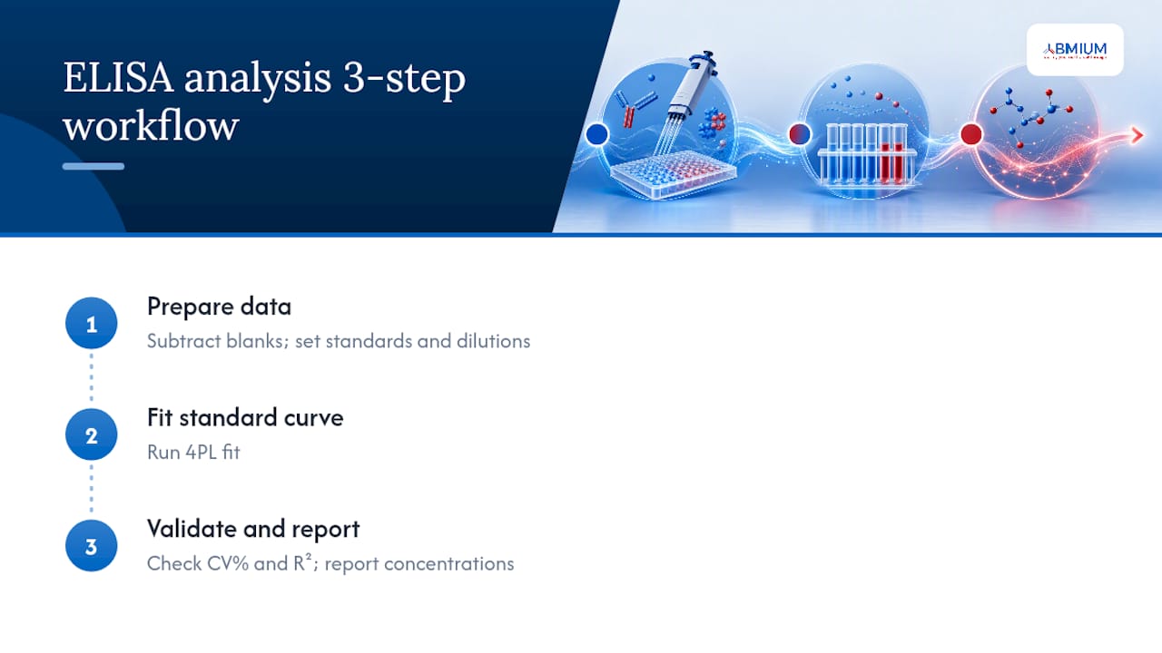
For most routine ELISA work, BeELISA and the elisa_4pl R Shiny app give you reproducible, free 4PL fitting, while browser tools like the Simulations4All analyser suit quick single-plate checks. The workflow behind every reliable result is the same three steps regardless of which tool you pick:
- Prepare: subtract blanks, format standards and replicates correctly
- Fit: run a 4PL (or 5PL if your curve is asymmetric) model against your standard curve
- Check: verify CV% and R² before you trust a single concentration value
Acceptance thresholds worth memorising: replicate CV% should sit at or below 15% (relaxing to 20% near the LLOQ), and your standard curve fit should return a high R² value before you back-calculate anything.
Key Takeaways
Accurate ELISA concentrations depend on correct blank subtraction, a properly chosen 4PL or 5PL fit, and CV%/R² checks run before any result is reported.
| Point | Details |
|---|---|
| Match tool to need | Use browser analysers for quick checks, R/Shiny apps like elisa_4pl for reproducible batches, and BeELISA for auditable desktop pipelines. |
| Format data first | Subtract blanks, use at least six calibrators, and keep dilution factors as separate numeric columns. |
| Fit with 4PL by default | Reserve 5PL for asymmetric curves, and never extrapolate beyond your calibrator range. |
| Verify with CV% and R² together | Flag replicate CV% above 15% to 20%. Confirm standard back-calculated accuracy within commonly recommended ranges. |
| Escalate reagent issues | When curves stay inconsistent despite correct analysis, ABMIUM’s verified antibodies and validation services address reagent-level causes. |
Table of Contents
- What are the best free ELISA data analysis tools?
- How do you format raw ELISA data before analysis?
- Should you use a 4PL or 5PL curve fit?
- What QC checks confirm your ELISA results are trustworthy?
- What pitfalls cause bad ELISA data analysis?
- What should you export from an ELISA analysis?
- Sources
- FAQ
What are the best free ELISA data analysis tools?
The right tool depends on how much reproducibility and audit trail your work demands, not just what fits on a browser tab. Three categories cover almost every use case a laboratory scientist encounters.
Browser-based analysers work best when you need a fast answer from a single plate and don’t need to retain a versioned pipeline. The Simulations4All ELISA Data Analyzer runs 4PL fitting directly in-browser, flags samples outside the LLOQ/ULOQ range, and reports CV% per point without installing anything. A similar tool from PunnettSquare shows the kind of output you should expect: fitted curves, R² values, and interactive controls for flagging out-of-range samples that need dilution or a re-run. These are ideal for teaching, pilot studies, or a same-day sanity check, but they typically lack batch processing or the metadata logging that regulated or multi-plate studies require.
Open-source R/Shiny apps suit labs that want reproducible, versioned analysis without paying for commercial software. The elisa_4pl Shiny app lets you upload an Excel file, run a 4PL fit, inspect residual plots, and download both the fitted parameters and plate plots. It expects specific column formatting, so following the app’s example input file matters more than you’d think.
Desktop pipelines answer a different need entirely: offline work, session persistence, or concerns about GxP and 21 CFR Part 11 traceability. BeELISA bundles raw OD import, standard curve fitting, back-calculation and automated QC into one auditable pipeline, with session save and restore built in.
- Browser tools: fastest, least setup, weakest audit trail
- R/Shiny apps: reproducible, scriptable, good for batches
- Desktop apps: best for offline, regulated, or high-volume work
How do you format raw ELISA data before analysis?
Most fit failures trace back to formatting, not the model itself. Tool documentation for elisa_4pl explicitly warns that skipping blank subtraction before analysis is one of the most common causes of invalid back-calculated concentrations.
- Subtract blank wells first. Average your blank replicates and subtract that value from every raw OD reading before it touches any fitting software. Document the blank value used, not just the corrected numbers.
- Design a plate layout that supports the model. Use multiple calibrator points, run standards and samples in duplicate or triplicate, and include a positive and negative control on every plate.
- Format your spreadsheet correctly. Most tools expect a specific column structure: sample ID, raw OD, dilution factor, and replicate number as separate columns, with standards clearly distinguished from unknowns.
- Record dilution factors as numeric multipliers, not text labels like “1 in 10”, and apply them only after back-calculation, never before the fit.
Pro Tip: Keep two separate files: one with raw, untouched OD values and a second with your blank-corrected data. When a fit looks wrong weeks later, you’ll want to trace exactly where the correction happened rather than guessing.
Should you use a 4PL or 5PL curve fit?
The four-parameter logistic (4PL) model is the industry standard for ELISA because the sigmoidal binding curve it describes matches how antibody-antigen interactions actually saturate at both ends. Best-practice guidance recommends 4PL as the default, reserving the five-parameter logistic (5PL) for curves that show clear asymmetry between the upper and lower asymptotes.
Both models require inversion to convert a measured OD back into a concentration, and that inversion is only valid within the standard curve’s own range. Extrapolating beyond your highest or lowest calibrator produces numbers that look precise but aren’t defensible.
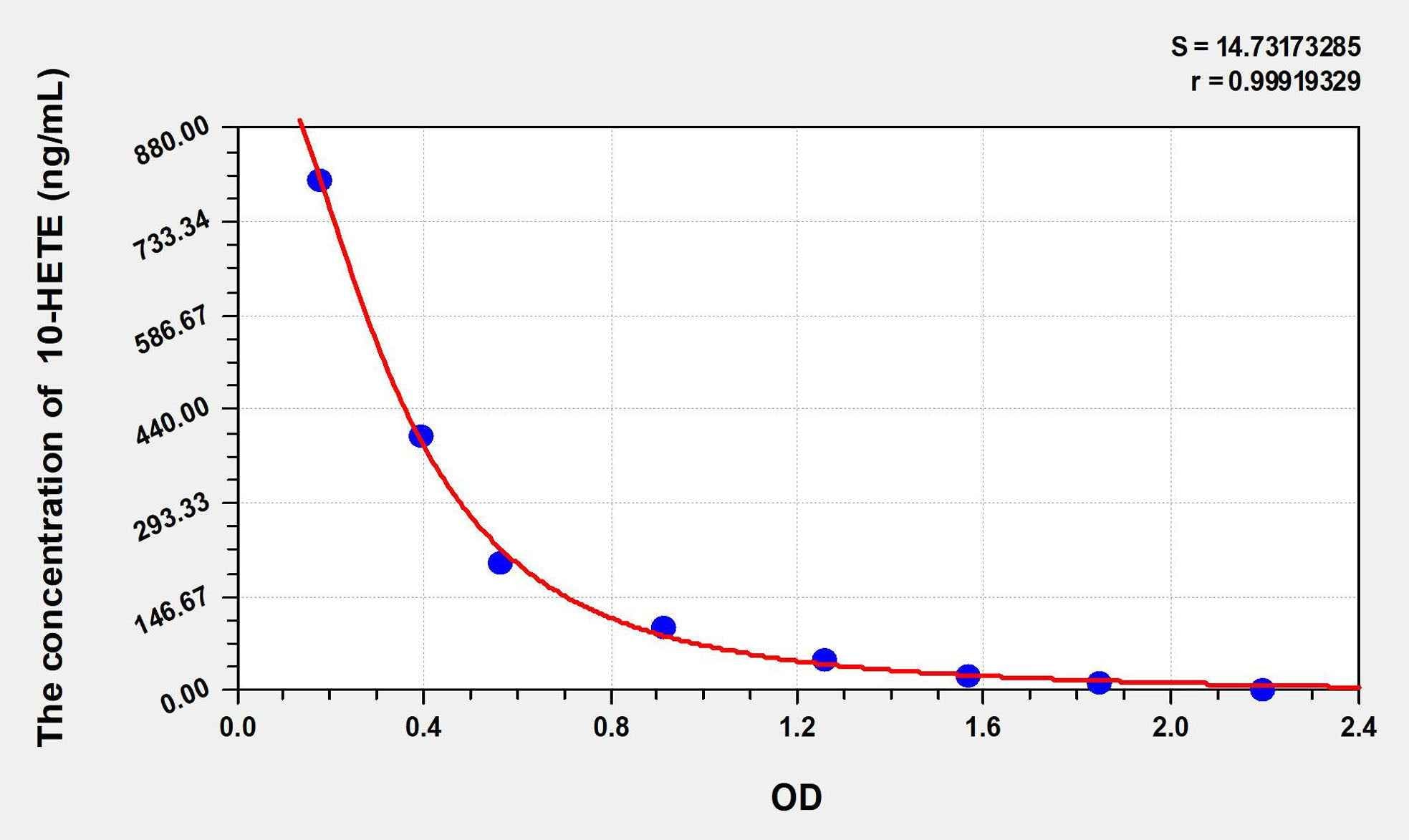
- Never trust R² in isolation. Simulation-based demonstrations show that a poor fit at the plate extremes can still return a deceptively high R² value.
- Always overlay the fitted curve on your raw points visually, and check the residual plot for systematic patterns rather than random scatter.
- Resist the temptation to force a polynomial fit for a “better” R². A 4PL or 5PL model reflects the biology; a polynomial does not, and it will interpolate badly near the edges.
A curve with R² above 0.99 can still fail on replicate agreement. Precision and goodness-of-fit are separate questions, and both need answering before you report a number.
What QC checks confirm your ELISA results are trustworthy?
Passing a curve fit is not the same as passing quality control. Run these checks on every plate before concentrations leave the lab.
- Calculate CV% for every replicate pair. Flag anything above 15%, or above 20% specifically for points near the lower limit of quantification, where variability naturally increases.
- Check standard back-calculated accuracy. Each calibrator, when its own OD is run back through the fitted curve, should recover within commonly recommended accuracy ranges, with most calibrators passing.
- Confirm your samples fall within the LLOQ and ULOQ. Anything outside that range needs dilution and a re-run rather than a reported number with a caveat attached.
- Inspect per-point CV and residuals together, not separately. A single high-CV point combined with a residual spike usually points to a pipetting error or edge-well evaporation effect rather than a biological signal.
- If a plate fails, don’t patch it. Dilute high samples and re-run, or repeat the standard curve with additional replicates before accepting any values from that plate.
What pitfalls cause bad ELISA data analysis?
The most common errors are procedural, not statistical. A missing dilution factor column, wells labelled inconsistently between the raw file and the analysis tool, or blanks that were never subtracted will all produce concentrations that look plausible and are wrong. Practitioners repeatedly find that a visually perfect curve with high R² can still hide poor replicate agreement, which is exactly why residuals and CV% deserve as much attention as the fit line itself.
Pro Tip: Save a template input file with your standard concentrations and plate layout pre-filled. Reusing it every time removes the single biggest source of formatting errors: retyping calibrator values from memory.
When a fit and a replicate check disagree, believe the replicate check. A curve is a mathematical approximation; your CV% tells you what actually happened on the bench.
Keeping a running plate log, noting kit lot and reader settings alongside each run, makes it far easier to spot when a pattern of failures points to a reagent problem rather than a technique problem. That’s usually the moment to move from a browser tool to a documented desktop pipeline, or to bring in independent validation.
What should you export from an ELISA analysis?
Reproducibility depends on keeping more than the final concentration table. Before you close a plate out, export and file:
- Raw OD values, untouched by any correction
- Blank-corrected OD values, saved separately
- Fitted curve parameters (4PL or 5PL coefficients) and the R² value
- The back-calculated concentration table with flagged out-of-range samples
- A plot image (PNG) of the fitted curve with data points overlaid
Record kit lot number, plate ID, reader settings, incubation times, and every dilution factor alongside these files, and version each export so a reviewer can trace exactly which run produced which number.
Free tools versus validated pipelines: Veron’s view
Free tools are entirely adequate for routine research, pilot studies, and internal decision-making, and there’s no reason to overcomplicate that work. Where the stakes rise, regulated submissions, high-value publications, or a reagent that keeps producing inconsistent curves, a validated pipeline or independent reagent validation earns its keep. ABMIUM’s scientific support exists precisely for that second scenario, not to replace the free workflow you already use.
A faster route to consistent ELISA results
Even the best curve-fitting workflow can’t rescue a plate run with an unreliable antibody. If you’ve traced inconsistent CV% or drifting standards back to reagent quality rather than analysis technique, ABMIUM’s catalogue of verified antibodies and ELISA kits is built to close that gap. Every antibody, including options like the Anti-Human CD135 antibody, carries reviewed provenance and pre-purchase validation data, so you spend less time re-running plates to rule out a bad lot.
For labs handling secondary detection variability, ABMIUM also lists validated conjugates such as the Anti-Mouse IgG antibody. When the analysis is solid but the results still look inconsistent, request a quote or browse the current catalogue to compare validated reagent options for your next assay run.
Sources
FAQ
How can I analyse ELISA data in Excel?
Excel can calculate blank-corrected OD values and basic CV%, but it cannot perform a proper 4PL or 5PL fit on its own. Export your formatted data to a free tool such as the elisa_4pl Shiny app for the actual curve fitting step.
How do I analyse ELISA data step by step?
Subtract blanks, format standards and samples with correct dilution columns, run a 4PL fit, then check CV% and R² before reporting any back-calculated concentration.
How do I fit an ELISA curve?
Plot OD against known standard concentrations and fit a four-parameter logistic model, which matches the sigmoidal shape of antibody binding better than a linear or polynomial fit. Confirm the fit visually and check residuals rather than relying on R² alone.
What CV% is acceptable for ELISA replicates?
A CV% at or below 15% is the general target, rising to a tolerance of 20% specifically near the lower limit of quantification, where variability naturally increases.